Time and Phase Alignment
This tutorial demonstrates how to use PyART to align waveforms in time and phase over a certain chosen time window.
%matplotlib inline
%config InlineBackend.figure_format = 'retina'

import numpy as np
import matplotlib.pyplot as plt
from matplotlib import rcParams
import seaborn as sns

# logging configuration, default INFO level
from PyART.logging_config import setup_logging
setup_logging()


# Set up Seaborn aesthetics
sns.set_context('talk')
sns.set_theme(font_scale=1.2)
sns.set_style('ticks')

# Update matplotlib rcParams
rcParams.update(
    {
        'text.usetex': False,
        'font.family': 'stixgeneral',
        'mathtext.fontset': 'stix',
        'axes.grid': True,
        'grid.linestyle': ':',
        'grid.color': '#bbbbbb',
        'axes.linewidth': 1,
    }
)
from PyART.catalogs import sxs, rit
from PyART.utils import utils, wf_utils
We first download two waveforms from the SXS and RIT catalogs, respectively. These waveforms correspond to the same physical system: a BBH targeted to GW150914 (see Lovelace et. al.)
def align_wfs(wf1, wf2, time_window=[1000, 2500], ref=None, N_interp=20000):
    """
    Align two waveforms based on the (2,2) mode.

    Parameters
    ----------
    wf1, wf2 : Waveform objects
        The two waveforms to be aligned.
    time_window : list, optional
        Time window [start, end] (in M) over which to perform the alignment.
        Default is [1000, 2500].
    ref : float, optional
        Reference time (in M) w.r.t. merger to align the waveforms. If provided, the alignment
        will be done at this time instead of over a time window. Default is None.
    N_interp : int, optional
        Number of points for interpolation when aligning over a time window. Default is 20000.
    Returns
    -------
    tau : float
        Time shift (in M) to apply to wf1 to align with wf2.
    dphi : float
        Phase shift (in radians) to apply to wf1 to align with wf2.
    """

    # align the (2,2) mode
    h22_1   = wf1.hlm[(2,2)]
    h22_2   = wf2.hlm[(2,2)]

    # extract waveform 1
    A_1, phi_1    = h22_1['A'], h22_1['p']
    u_1           = wf1.u
    imrg_1        = np.argmax(A_1)
    u_1_mrg       = u_1[imrg_1]

    # extract waveform 2
    A_2, phi_2   = h22_2['A'], h22_2['p']
    u_2          = wf2.u
    imrg_2       = np.argmax(A_2)
    u_2_mrg      = u_2[imrg_2]

    # shift mergers to same point
    u_1 = u_1 - u_1_mrg + u_2_mrg
    tau = - u_1_mrg + u_2_mrg

    if ref is not None:
        # align at reference time w.r.t merger
        t_mrg_1 = u_1[imrg_1]
        t_mrg_2 = u_2[imrg_2]
        i_ref_1 = utils.find_nearest(t_mrg_1+ref, u_1)
        i_ref_2 = utils.find_nearest(t_mrg_2+ref, u_2)
        dphi = phi_1[i_ref_1] - phi_2[i_ref_2]
        dtau  = u_2[i_ref_2] - u_1[i_ref_1]
    else:
        # common time array
        u_new = np.linspace(max(u_1[0], u_2[0]), min(u_1[-1], u_2[-1]), N_interp)

        win_start = u_2[utils.find_nearest(time_window[0], u_2)]
        win_end   = u_2[utils.find_nearest(time_window[1], u_2)]

        dtau , dphi , _ = wf_utils.Align(u_new, win_end , win_end-win_start , u_1, phi_1, u_2, phi_2)

    tau += dtau

    return tau, dphi
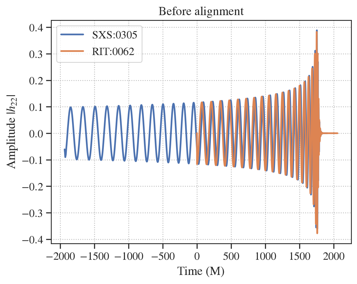
# Waveforms
wf_sxs = sxs.Waveform_SXS(ID='0305', path='./', download=True, downloads=['hlm', 'metadata'], nu_rescale=False)
wf_rit = rit.Waveform_RIT(ID='0062', path='./', download=True, nu_rescale=False)

# pre-shift SXS to RIT merger time
wf_sxs._u -= wf_sxs.u[0]
wf_rit._u -= wf_rit.u[0]
t_mrg_rit, *_ = wf_rit.find_max()
t_mrg_sxs, *_ = wf_sxs.find_max()
wf_sxs._u += (t_mrg_rit - t_mrg_sxs)

# window for alignment
time_window = [500, 1000]

# plot the waveforms before alignment
fig, ax = plt.subplots()
ax.plot(wf_sxs.u, wf_sxs.hlm[(2,2)]['real'], label='SXS:0305', lw=2)
ax.plot(wf_rit.u, wf_rit.hlm[(2,2)]['real'], label='RIT:0062', lw=2)
ax.set_xlabel('Time (M)')
ax.set_ylabel(r'Amplitude $|h_{22}|$')
ax.legend()
ax.set_title('Before alignment')
plt.show()

# Align the two waveforms
tau, dphi = align_wfs(wf_rit, wf_sxs, time_window=time_window)
wf_rit._u += tau
print(f"Time shift (M): {tau:.2f}")
print(f"Phase shift (rad): {dphi:.2f}")
2026-06-17 15:28:02 The path ./SXS_BBH_0305 does not exist or contains no 'Lev*' directory.
2026-06-17 15:28:02 Downloading the simulation from the SXS catalog.
2026-06-17 15:28:03 Setting the download (cache) directory to ./
2026-06-17 15:28:12 Loaded SXS simulation SXS:BBH:0305.
2026-06-17 15:28:14 Saved hlm data.
2026-06-17 15:28:14 Saved metadata.
2026-06-17 15:28:14 The path ./RIT_BBH_0062 does not exist.
2026-06-17 15:28:14 Downloading the simulation from the RIT catalog.
2026-06-17 15:28:14 JSON file with RIT urls not found, fetching and parsing catalog webpage: https://ccrgpages.rit.edu/~RITCatalog/
2026-06-17 15:28:20 Created JSON file with RIT urls: /opt/hostedtoolcache/Python/3.11.15/x64/lib/python3.11/site-packages/PyART/catalogs/rit_urls.json
2026-06-17 15:28:20 --------------------------------------------------
2026-06-17 15:28:20 Downloading RIT:BBH:0062
2026-06-17 15:28:20 --------------------------------------------------
2026-06-17 15:28:20 wget-ing https://ccrgpages.rit.edu/~RITCatalog/Metadata/RIT:BBH:0062-n120-id3_Metadata.txt ...
2026-06-17 15:28:21 wget-ing https://ccrgpages.rit.edu/~RITCatalog/Data/ExtrapPsi4_RIT-BBH-0062-n120-id3.tar.gz ...
2026-06-17 15:28:21 Extracting ExtrapPsi4_RIT-BBH-0062-n120-id3.tar.gz ...
2026-06-17 15:28:22 wget-ing https://ccrgpages.rit.edu/~RITCatalog/Data/ExtrapStrain_RIT-BBH-0062-n120.h5 ...
2026-06-17 15:28:22 >> Elapsed time: 1.585 s
Time shift (M): -0.29
Phase shift (rad): -55.53
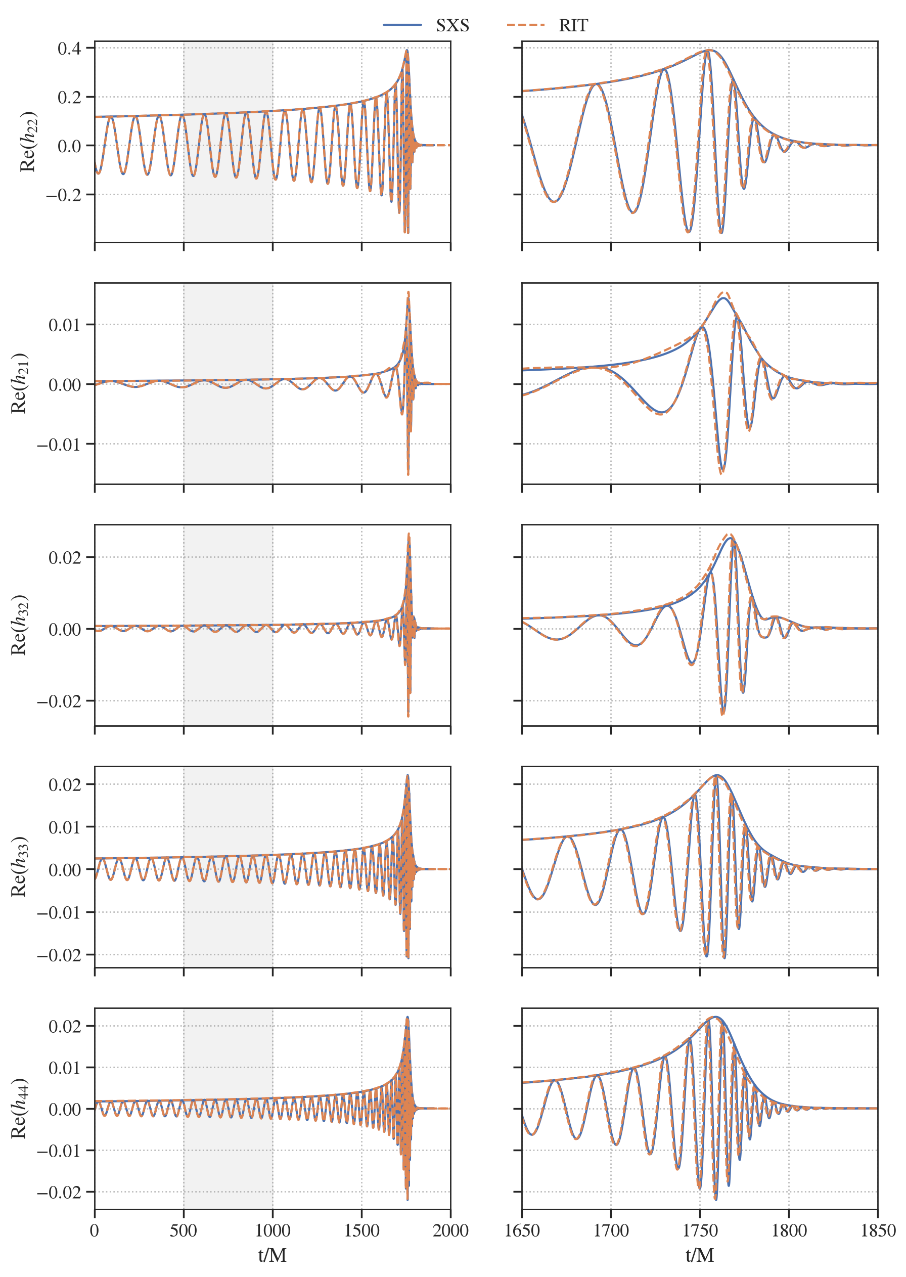
# propagate phase shift to all modes

modes = [(2,2), (2,1), (3,2), (3,3), (4,4)]

fig, ax = plt.subplots(len(modes), 2, figsize=(10, 3*len(modes)), sharex='col', sharey='row')
for j, (l, m) in enumerate(modes):

    # note: the 2pi shift is sometimes required to get correct sign for odd-m modes
    this_dphi = (dphi + 2*np.pi)*m / 2

    h_lm = wf_rit.hlm[(l,m)]['z']
    h_lm_shifted = h_lm * np.exp(1j * this_dphi)

    # Plotting
    for col in range(2):
        ax[j, col].plot(wf_sxs.u, wf_sxs.hlm[(l,m)]['real'], label='SXS', color='C0', linestyle='-')
        ax[j, col].plot(wf_rit.u, np.real(h_lm_shifted), label='RIT', color='C1', linestyle='--')
        ax[j, col].plot(wf_sxs.u, wf_sxs.hlm[(l,m)]['A'],color='C0', linestyle='-')
        ax[j, col].plot(wf_rit.u, np.abs(h_lm_shifted), color='C1', linestyle='--')

    ax[j, 0].set_ylabel(r'Re$(h_{%d%d})$' % (l, m))
    ax[j, 0].axvspan(time_window[0], time_window[1], color='gray', alpha=0.1)

ax[-1, 0].set_xlabel('t/M')
ax[-1, 0].set_xlim(0, 2000)
ax[-1, 1].set_xlabel('t/M')
ax[-1, 1].set_xlim(1650, 1850)

# legend on top of the figure
ax[0, 0].legend(loc='upper center', bbox_to_anchor=(1.1, 1.2), ncol=2, frameon=False)

plt.show()