Intro to Waveforms
This tutorial demonstrates how to use PyART’s waveform class
%matplotlib inline
%config InlineBackend.figure_format = 'retina'

import numpy as np
import matplotlib.pyplot as plt
from matplotlib import rcParams
import seaborn as sns

# logging configuration, default INFO level
from PyART.logging_config import setup_logging
setup_logging()

# Set up Seaborn aesthetics
sns.set_context('talk')
sns.set_theme(font_scale=1.2)
sns.set_style('ticks')

# Update matplotlib rcParams
rcParams.update(
    {
        'text.usetex': False,
        'font.family': 'stixgeneral',
        'mathtext.fontset': 'stix',
        'axes.grid': True,
        'grid.linestyle': ':',
        'grid.color': '#bbbbbb',
        'axes.linewidth': 1,
    }
)
We now create an empty Waveform object and inspect its attributes.
This class is inherited by all waveform catalogs and models, meaning that they will all have these attributes and methods.
For more information, see the Waveform class documentation.
from PyART.waveform import Waveform

# Create an empty Waveform object
waveform = Waveform()

attributes = [attr for attr in dir(waveform) if not attr.startswith('_') and not callable(getattr(waveform, attr))]
methods = [method for method in dir(waveform) if not method.startswith('_') and callable(getattr(waveform, method))]

print("Attributes of the Waveform object:")
for attr in attributes:
    print(f"- {attr}")

print("\nMethods of the Waveform object:")
for method in methods:
    print(f"- {method}")
Attributes of the Waveform object:
- domain
- dothlm
- dyn
- f
- hc
- hlm
- hp
- kind
- psi4lm
- t
- t_psi4
- u
- units

Methods of the Waveform object:
- compute_dothlm
- compute_hphc
- compute_psi4lm
- cut
- dynamics_from_hlm
- ej_from_hlm
- find_max
- integrate_data
- interpolate_hlm
- phase_shift
- to_SI
- to_frequency
- to_geom
- to_time
We now load a waveform from the SXS catalog and plot its modes \(h_{\ell m}\).
They are stored as a dictionary of the form: hlm[(l,m)]. Each dictionary entry has the amplitude: A and phase p of the mode, as well as the real and imag part of \(h_{\ell,m}\).
Note that, by default, the modes are not interpolated to a uniform time grid. Therefore, before plotting, we:
Interpolate to a uniform time grid with
waveform.interpolate_hlmShift the time array so that the (2,2) mode peaks at \(t=0M\), using the
find_maxmethod.
from PyART.catalogs import sxs

# Utility function to check if an array is uniformly spaced
def is_uniform(arr, rtol=1e-10, atol=1e-12):
    delta = np.diff(arr)
    return np.allclose(delta, delta[0], rtol=rtol, atol=atol)

sxs_waveform = sxs.Waveform_SXS(ID='0180',
                                download=True,
                                ignore_deprecation=True,
                                downloads=["hlm", "metadata", "horizons"],
                                load=["hlm", "metadata", "horizons"]
                                )


# verify that the time array is uniform
print("Is the time array uniform?", is_uniform(sxs_waveform.u))

# interpolate to uniform time gri, dT = 1M
t_interp, hlm_interp = sxs_waveform.interpolate_hlm(1)

# overwrite time array and modes in the waveform object
sxs_waveform._t = t_interp
sxs_waveform._u = t_interp
sxs_waveform._hlm = hlm_interp

# verify that the time array is uniform
print("Is the time array uniform?", is_uniform(sxs_waveform.u))

t_max, _, _, _, mrg_idx = sxs_waveform.find_max(return_idx=True, mode=(2,2))

fig, ax = plt.subplots()
modes = [(2, 2), (2, 1), (3, 3), (4, 4), (2, -2), (2, -1), (3, -3), (4, -4)]
for mode in modes:
    ax.semilogy(sxs_waveform.u-t_max, sxs_waveform.hlm[mode]['A'], label=f'{mode}')

# legend, out of box
ax.legend(ncol=1, bbox_to_anchor=(1.05, 1), loc='upper left')
ax.axvline(0, color='k', linestyle='--', alpha=0.5)
ax.set_xlabel('t/M')
ax.set_ylabel(r'$h_{\ell m}/\nu$')
plt.show()
2026-06-17 15:27:05 The path ../dat/SXS/SXS_BBH_0180 does not exist or contains no 'Lev*' directory.
2026-06-17 15:27:05 Downloading the simulation from the SXS catalog.
2026-06-17 15:27:06 Setting the download (cache) directory to ../dat/SXS/
2026-06-17 15:27:17 Loaded SXS simulation SXS:BBH:0180.
2026-06-17 15:27:30 Saved hlm data.
2026-06-17 15:27:34 Saved horizons data.
2026-06-17 15:27:34 Saved metadata.
Is the time array uniform? False
Is the time array uniform? True
---------------------------------------------------------------------------
AttributeError                            Traceback (most recent call last)
File /opt/hostedtoolcache/Python/3.11.15/x64/lib/python3.11/site-packages/PIL/ImageFile.py:663, in _save(im, fp, tile, bufsize)
    662 try:
--> 663     fh = fp.fileno()
    664     fp.flush()

AttributeError: '_idat' object has no attribute 'fileno'

During handling of the above exception, another exception occurred:

KeyboardInterrupt                         Traceback (most recent call last)
Cell In[3], line 42
     38 ax.legend(ncol=1, bbox_to_anchor=(1.05, 1), loc='upper left')
     39 ax.axvline(0, color='k', linestyle='--', alpha=0.5)
     40 ax.set_xlabel('t/M')
     41 ax.set_ylabel(r'$h_{\ell m}/\nu$')
---> 42 plt.show()

File /opt/hostedtoolcache/Python/3.11.15/x64/lib/python3.11/site-packages/matplotlib/pyplot.py:646, in show(*args, **kwargs)
    602 """
    603 Display all open figures.
    604
   (...)    643 explicitly there.
    644 """
    645 _warn_if_gui_out_of_main_thread()
--> 646 return _get_backend_mod().show(*args, **kwargs)

File /opt/hostedtoolcache/Python/3.11.15/x64/lib/python3.11/site-packages/matplotlib_inline/backend_inline.py:90, in show(close, block)
     88 try:
     89     for figure_manager in Gcf.get_all_fig_managers():
---> 90         display(
     91             figure_manager.canvas.figure,
     92             metadata=_fetch_figure_metadata(figure_manager.canvas.figure),
     93         )
     94 finally:
     95     show._to_draw = []

File /opt/hostedtoolcache/Python/3.11.15/x64/lib/python3.11/site-packages/decorator/__init__.py:247, in decorate.<locals>.fun(*args, **kw)
    245 if not kwsyntax:
    246     args, kw = fix(args, kw, sig)
--> 247 return caller(func, *(extras + args), **kw)

File /opt/hostedtoolcache/Python/3.11.15/x64/lib/python3.11/site-packages/matplotlib/backend_bases.py:2281, in FigureCanvasBase.print_figure(self, filename, dpi, facecolor, edgecolor, orientation, format, bbox_inches, pad_inches, bbox_extra_artists, backend, **kwargs)
   2277 try:
   2278     # _get_renderer may change the figure dpi (as vector formats
   2279     # force the figure dpi to 72), so we need to set it again here.
   2280     with cbook._setattr_cm(self.figure, dpi=dpi):
-> 2281         result = print_method(
   2282             filename,
   2283             facecolor=facecolor,
   2284             edgecolor=edgecolor,
   2285             orientation=orientation,
   2286             bbox_inches_restore=_bbox_inches_restore,
   2287             **kwargs)
   2288 finally:
   2289     if bbox_inches and restore_bbox:

File /opt/hostedtoolcache/Python/3.11.15/x64/lib/python3.11/site-packages/matplotlib/backend_bases.py:2138, in FigureCanvasBase._switch_canvas_and_return_print_method.<locals>.<lambda>(*args, **kwargs)
   2134     optional_kws = {  # Passed by print_figure for other renderers.
   2135         "dpi", "facecolor", "edgecolor", "orientation",
   2136         "bbox_inches_restore"}
   2137     skip = optional_kws - {*inspect.signature(meth).parameters}
-> 2138     print_method = functools.wraps(meth)(lambda *args, **kwargs: meth(
   2139         *args, **{k: v for k, v in kwargs.items() if k not in skip}))
   2140 else:  # Let third-parties do as they see fit.
   2141     print_method = meth

File /opt/hostedtoolcache/Python/3.11.15/x64/lib/python3.11/site-packages/matplotlib/backends/backend_agg.py:537, in FigureCanvasAgg.print_png(self, filename_or_obj, metadata, pil_kwargs)
    490 def print_png(self, filename_or_obj, *, metadata=None, pil_kwargs=None):
    491     """
    492     Write the figure to a PNG file.
    493
   (...)    535         *metadata*, including the default 'Software' key.
    536     """
--> 537     self._print_pil(filename_or_obj, "png", pil_kwargs, metadata)

File /opt/hostedtoolcache/Python/3.11.15/x64/lib/python3.11/site-packages/matplotlib/backends/backend_agg.py:486, in FigureCanvasAgg._print_pil(self, filename_or_obj, fmt, pil_kwargs, metadata)
    481 """
    482 Draw the canvas, then save it using `.image.imsave` (to which
    483 *pil_kwargs* and *metadata* are forwarded).
    484 """
    485 FigureCanvasAgg.draw(self)
--> 486 mpl.image.imsave(
    487     filename_or_obj, self.buffer_rgba(), format=fmt, origin="upper",
    488     dpi=self.figure.dpi, metadata=metadata, pil_kwargs=pil_kwargs)

File /opt/hostedtoolcache/Python/3.11.15/x64/lib/python3.11/site-packages/matplotlib/image.py:1722, in imsave(fname, arr, vmin, vmax, cmap, format, origin, dpi, metadata, pil_kwargs)
   1720 pil_kwargs.setdefault("format", format)
   1721 pil_kwargs.setdefault("dpi", (dpi, dpi))
-> 1722 image.save(fname, **pil_kwargs)

File /opt/hostedtoolcache/Python/3.11.15/x64/lib/python3.11/site-packages/PIL/Image.py:2713, in Image.save(self, fp, format, **params)
   2710     fp = cast(IO[bytes], fp)
   2712 try:
-> 2713     save_handler(self, fp, filename)
   2714 except Exception:
   2715     if open_fp:

File /opt/hostedtoolcache/Python/3.11.15/x64/lib/python3.11/site-packages/PIL/PngImagePlugin.py:1507, in _save(im, fp, filename, chunk, save_all)
   1505 if single_im:
   1506     _apply_encoderinfo(single_im, im.encoderinfo)
-> 1507     ImageFile._save(
   1508         single_im,
   1509         cast(IO[bytes], _idat(fp, chunk)),
   1510         [ImageFile._Tile("zip", (0, 0) + single_im.size, 0, rawmode)],
   1511     )
   1513 if info:
   1514     for info_chunk in info.chunks:

File /opt/hostedtoolcache/Python/3.11.15/x64/lib/python3.11/site-packages/PIL/ImageFile.py:667, in _save(im, fp, tile, bufsize)
    665     _encode_tile(im, fp, tile, bufsize, fh)
    666 except (AttributeError, io.UnsupportedOperation) as exc:
--> 667     _encode_tile(im, fp, tile, bufsize, None, exc)
    668 if hasattr(fp, "flush"):
    669     fp.flush()

File /opt/hostedtoolcache/Python/3.11.15/x64/lib/python3.11/site-packages/PIL/ImageFile.py:693, in _encode_tile(im, fp, tile, bufsize, fh, exc)
    690 if exc:
    691     # compress to Python file-compatible object
    692     while True:
--> 693         errcode, data = encoder.encode(bufsize)[1:]
    694         fp.write(data)
    695         if errcode:

KeyboardInterrupt:
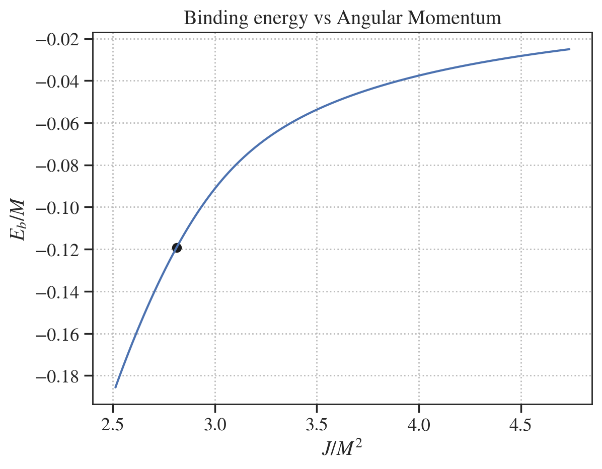
We now use the modes to compute the energy and angular momentum radiated as a function of time.
To do so we use the ej_from_hlm method of the Waveform class.
Note that this method requires knowledge of the initial ADM mass and angular momentum of the system, which are stored as attributes of the Waveform object (and automatically loaded, for most catalogs).
M_adm_0 = sxs_waveform.metadata['E0byM']
J_adm_0 = sxs_waveform.metadata['Jz0']
m1 = sxs_waveform.metadata['m1']
m2 = sxs_waveform.metadata['m2']

eb, e, jorb = sxs_waveform.ej_from_hlm(M_adm_0, J_adm_0, m1, m2, modes=modes)

# identify merger
e_mrg = eb[mrg_idx]
j_mrg = jorb[mrg_idx]

fig, ax = plt.subplots()
ax.plot(jorb, eb)
ax.set_xlabel(r'$J/M^2$')
ax.set_ylabel(r'$E_b/M$')
ax.scatter(j_mrg, e_mrg, color='k', label='Merger')
ax.set_title('Binding energy vs Angular Momentum')
plt.show()
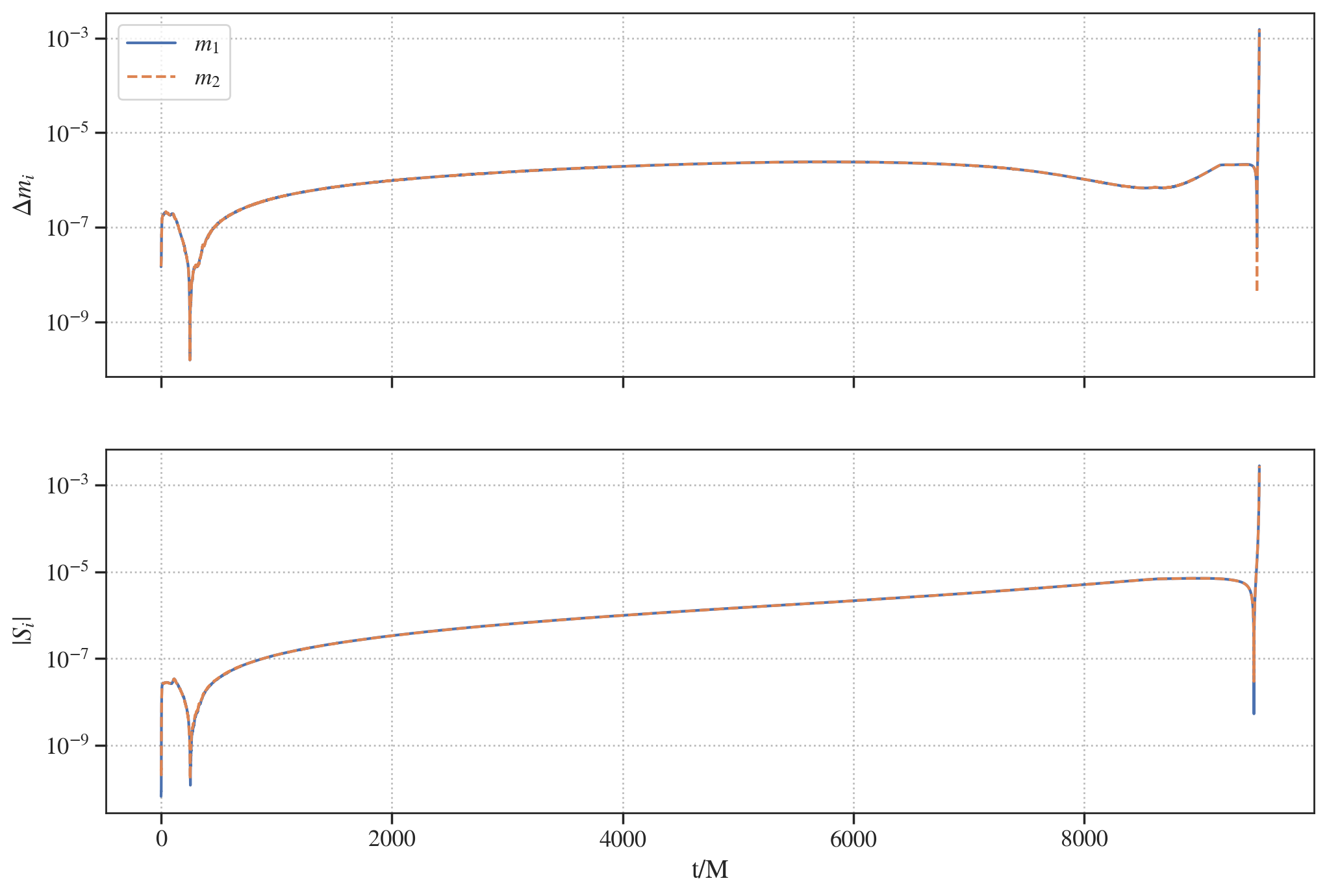
We will now look at the dynamics. This is not available for all catalogs/models. In the case of SXS waveforms, we do load Horizon data when we download the waveform and can access it.
# plot the mass / spin evolution
fig, axs = plt.subplots(2, 1, figsize=(12, 8), sharex=True)
axs[0].semilogy(sxs_waveform.dyn['t'], abs(sxs_waveform.dyn['m1']-m1), label=r'$m_1$')
axs[0].semilogy(sxs_waveform.dyn['t'], abs(sxs_waveform.dyn['m2']-m2), label=r'$m_2$', linestyle='--')
axs[1].semilogy(sxs_waveform.dyn['t'], sxs_waveform.dyn['chi1'], label=r'S_1')
axs[1].semilogy(sxs_waveform.dyn['t'], sxs_waveform.dyn['chi2'], label=r'S_2', linestyle='--')
axs[0].set_ylabel(r'$\Delta m_i$')
axs[1].set_ylabel(r'$|S_i|$')
axs[1].set_xlabel('t/M')
axs[0].legend()
plt.show()
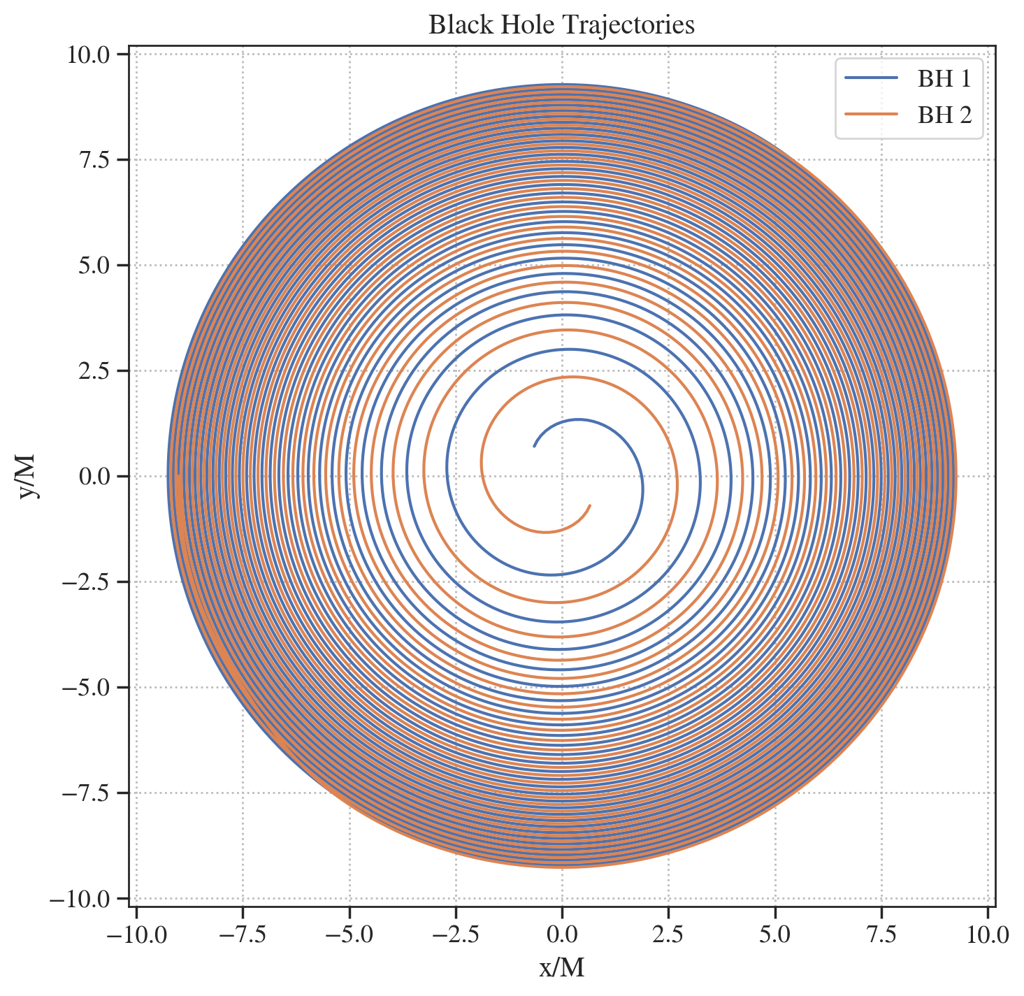
# plot the trajectories
xA = sxs_waveform.dyn['x1']
xB = sxs_waveform.dyn['x2']
fig, ax = plt.subplots(figsize=(8, 8))
ax.plot(xA[:, 0], xA[:, 1], label='BH 1')
ax.plot(xB[:, 0], xB[:, 1], label='BH 2')
ax.set_xlabel('x/M')
ax.set_ylabel('y/M')
ax.set_title('Black Hole Trajectories')
ax.legend()
plt.show()