Computing Mismatches Between NR and EOB Waveforms
This tutorial demonstrates how to compute frequency-domain mismatches between Numerical Relativity (NR) waveforms and Effective One Body (EOB) model waveforms.
The mismatch quantifies how well an EOB model reproduces an NR waveform, accounting for:
Time and phase shifts
Total binary mass
Initial frequency
TODO: add references and extend example to higher modes
Setup
%matplotlib inline
%config InlineBackend.figure_format = 'retina'

import numpy as np
import matplotlib.pyplot as plt
from PyART.catalogs import sxs
from PyART.models import teob
from PyART.analysis.match import Matcher
from PyART.utils import utils as ut
import time
WARNING: TEOBResumS not installed.
/opt/hostedtoolcache/Python/3.11.15/x64/lib/python3.11/site-packages/PyART/analysis/match.py:15: UserWarning: Wswiglal-redir-stdio:

SWIGLAL standard output/error redirection is enabled in IPython.
This may lead to performance penalties. To disable locally, use:

with lal.no_swig_redirect_standard_output_error():
    ...

To disable globally, use:

lal.swig_redirect_standard_output_error(False)

Note however that this will likely lead to error messages from
LAL functions being either misdirected or lost when called from
Jupyter notebooks.

To suppress this warning, use:

import warnings
warnings.filterwarnings("ignore", "Wswiglal-redir-stdio")
import lal

  import lal
Load NR Waveform from SXS
First, we load a numerical relativity waveform from the SXS catalog:
# Load SXS waveform
sxs_id = '0180'
nr = sxs.Waveform_SXS(
    path='./',
    download=True,
    ID=sxs_id,
    order="Extrapolated_N3.dir",
    ellmax=7,
    ignore_deprecation=True
)
nr.cut(300)  # Remove junk radiation

# Extract metadata
q = nr.metadata['q']
M = nr.metadata['M']
chi1z = nr.metadata['chi1z']
chi2z = nr.metadata['chi2z']
f0 = nr.metadata['f0']

print('==============================')
print(f'Mismatch for SXS:{sxs_id}')
print('==============================')
print(f'Mass ratio q : {q:.5f}')
print(f'Total mass M : {M:.5f}')
print(f'chi1z        : {chi1z:.5f}')
print(f'chi2z        : {chi2z:.5f}')
print(f'f0           : {f0:.5f}')
print('==============================')
==============================
Mismatch for SXS:0180
==============================
Mass ratio q : 1.00000
Total mass M : 1.00000
chi1z        : -0.00000
chi2z        : -0.00000
f0           : 0.00390
==============================
Generate Corresponding EOB Waveform
Now we generate an EOB waveform with the same parameters:
# EOB parameters
srate = 8192
eobpars = {
    'M': M,
    'q': q,
    'chi1': chi1z,
    'chi2': chi2z,
    'LambdaAl2': 0.,
    'LambdaBl2': 0.,
    'distance': 1.,
    'initial_frequency': 0.9*f0,
    'use_geometric_units': "yes",
    'interp_uniform_grid': "yes",
    'domain': 0,
    'srate_interp': srate,
    'inclination': 0.,
    'output_hpc': "no",
    'use_mode_lm': [1],
    'arg_out': "yes",
    'ecc': 1e-8,
    'coalescence_angle': 0.,
}

eob = teob.Waveform_EOB(pars=eobpars)
eob = eob * (q/(1+q)**2)

print("EOB waveform generated successfully")
---------------------------------------------------------------------------
NameError                                 Traceback (most recent call last)
Cell In[3], line 24
     20     'ecc': 1e-8,
     21     'coalescence_angle': 0.,
     22 }
     23
---> 24 eob = teob.Waveform_EOB(pars=eobpars)
     25 eob = eob * (q/(1+q)**2)
     26
     27 print("EOB waveform generated successfully")

File /opt/hostedtoolcache/Python/3.11.15/x64/lib/python3.11/site-packages/PyART/models/teob.py:34, in Waveform_EOB.__init__(self, pars)
     31 else:
     32     self._units = "SI"
---> 34 self._run_py()
     35 pass

File /opt/hostedtoolcache/Python/3.11.15/x64/lib/python3.11/site-packages/PyART/models/teob.py:70, in Waveform_EOB._run_py(self)
     68     self._domain = "Freq"
     69 else:
---> 70     t, hp, hc, hlm, dyn = EOB.EOBRunPy(self.pars)
     71     self._u = t
     72     hlm_conv = convert_hlm(hlm)

NameError: name 'EOB' is not defined
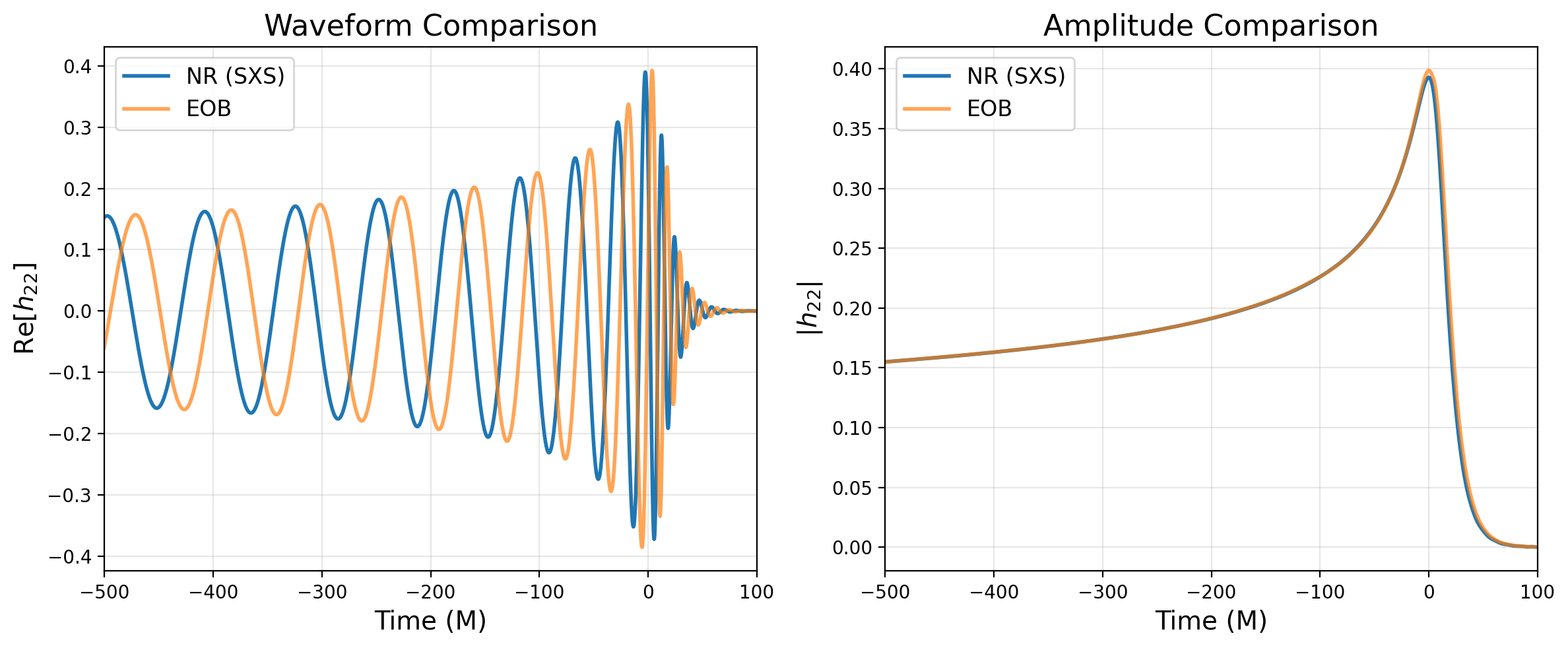
Visualize Waveforms
Let’s compare the NR and EOB waveforms visually:
# Find merger times
nr_mrg, _, _, _ = nr.find_max()
eob_mrg, _, _, _ = eob.find_max()

# Plot
plt.figure(figsize=(12, 5))

plt.subplot(1, 2, 1)
plt.plot(nr.u - nr_mrg, nr.hlm[(2,2)]['real'], label='NR (SXS)', linewidth=2)
plt.plot(eob.u - eob_mrg, eob.hlm[(2,2)]['real'], label='EOB', linewidth=2, alpha=0.7)
plt.xlabel('Time (M)', fontsize=14)
plt.ylabel(r'Re[$h_{22}$]', fontsize=14)
plt.title('Waveform Comparison', fontsize=16)
plt.legend(fontsize=12)
plt.grid(True, alpha=0.3)
plt.xlim([-500, 100])

plt.subplot(1, 2, 2)
plt.plot(nr.u - nr_mrg, nr.hlm[(2,2)]['A'], label='NR (SXS)', linewidth=2)
plt.plot(eob.u - eob_mrg, eob.hlm[(2,2)]['A'], label='EOB', linewidth=2, alpha=0.7)
plt.xlabel('Time (M)', fontsize=14)
plt.ylabel(r'$|h_{22}|$', fontsize=14)
plt.title('Amplitude Comparison', fontsize=16)
plt.legend(fontsize=12)
plt.grid(True, alpha=0.3)
plt.xlim([-500, 100])

plt.tight_layout()
plt.show()
Compute Mismatch vs Total Mass
The mismatch depends on the total mass of the binary because:
Different masses correspond to different frequency ranges
The detector sensitivity varies with frequency
Note that by default the mismatch is computed with the aLIGOZeroDetHighPower noise curve. You can change this by specifying a different noise curve in the settings dictionary.
Let’s compute the mismatch for a range of total masses:
# Define mass range
mass_min = 10   # Msun
mass_max = 200  # Msun
mass_num = 20
masses = np.linspace(mass_min, mass_max, num=mass_num)
mm = np.zeros_like(masses)

# Compute mismatches
t0 = time.perf_counter()
for i, M_total in enumerate(masses):
    f0_mm = 1.25 * f0 / (M_total * ut.Msun)

    matcher = Matcher(
        nr, eob,
        settings={
            'pre_align': True,
            'initial_frequency_mm': f0_mm,
            'final_frequency_mm': 2048,
            'tlen': len(nr.u),
            'dt': 1/srate,
            'M': M_total,
            'resize_factor': 4,
            'modes-or-pol': 'modes',
            'modes': [(2,2)],
            'pad_end_frac': 0.5,
            'taper_alpha': 0.20,
            'taper_start': 0.05,
            'taper': 'sigmoid',
            'cut_longer': True,
        }
    )
    mm[i] = matcher.mismatch

    if i % 5 == 0:
        print(f'M = {M_total:6.1f} Msun, f0 = {f0_mm:7.4f} Hz, mismatch = {mm[i]:.3e}')

elapsed = time.perf_counter() - t0
print(f'\nTotal elapsed time: {elapsed:.2f} seconds')
M =   10.0 Msun, f0 = 99.0953 Hz, mismatch = 5.795e-05
M =   60.0 Msun, f0 = 16.5159 Hz, mismatch = 1.176e-04
M =  110.0 Msun, f0 =  9.0087 Hz, mismatch = 1.253e-04
M =  160.0 Msun, f0 =  6.1935 Hz, mismatch = 1.234e-04

Total elapsed time: 10.42 seconds
Plot Mismatch vs Mass
plt.figure(figsize=(10, 6))
plt.plot(masses, mm, linewidth=2, marker='o', markersize=5)
plt.yscale('log')
plt.xlabel(r'Total Mass $M$ [$M_\odot$]', fontsize=16)
plt.ylabel(r'Mismatch $\bar{\mathcal{F}}$', fontsize=16)
plt.title(f'NR-EOB Mismatch for SXS:{sxs_id}', fontsize=18)
plt.ylim(1e-5, 1e-3)
plt.grid(True, alpha=0.3)
plt.tight_layout()
plt.show()

# Report statistics
print(f'Minimum mismatch: {mm.min():.3e} at M = {masses[mm.argmin()]:.1f} Msun')
print(f'Maximum mismatch: {mm.max():.3e} at M = {masses[mm.argmax()]:.1f} Msun')
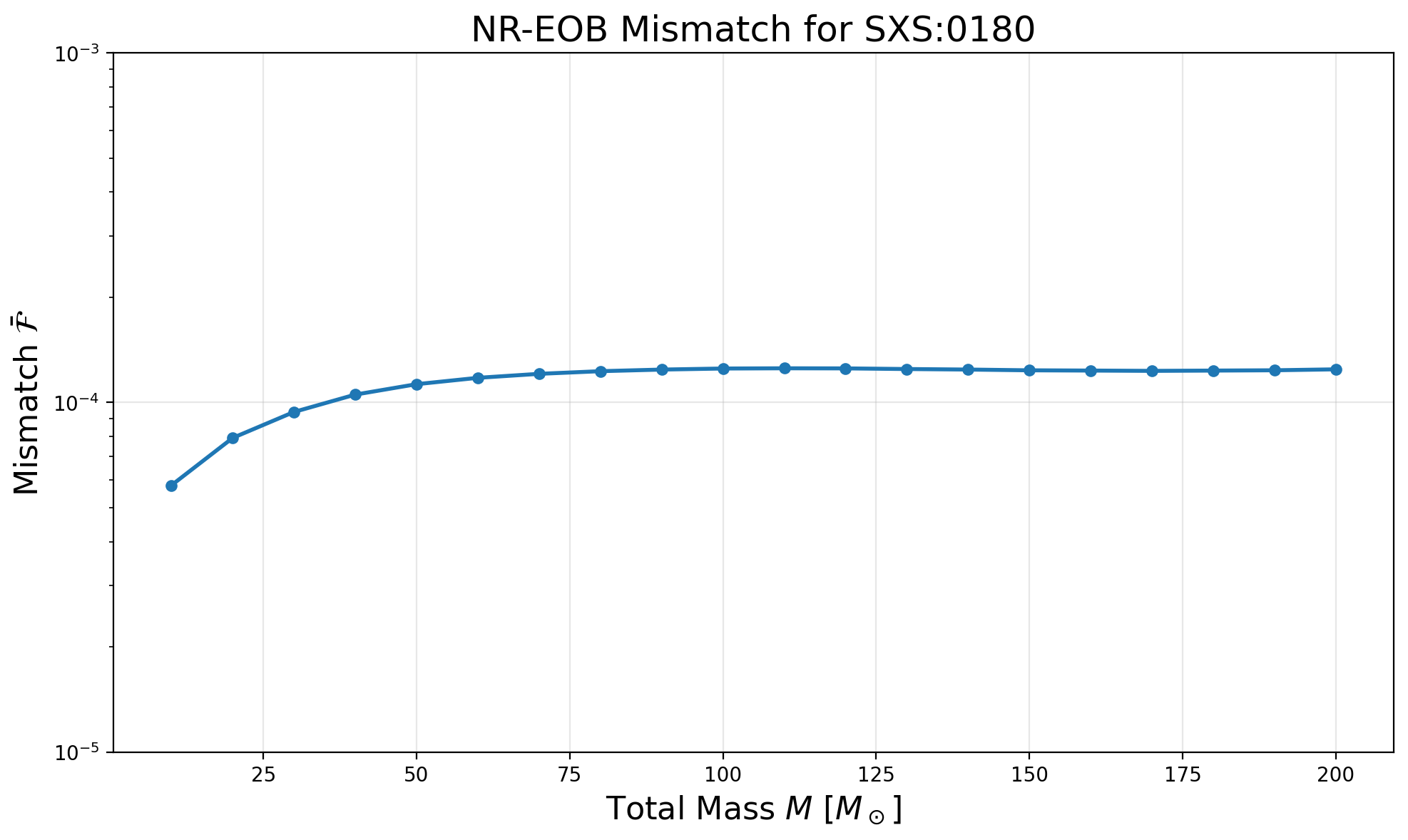
Minimum mismatch: 5.797e-05 at M = 10.0 Msun
Maximum mismatch: 1.253e-04 at M = 110.0 Msun
Summary
This tutorial demonstrated:
Loading NR waveforms from the SXS catalog
Generating corresponding EOB waveforms with matching parameters
Visualizing and comparing NR and EOB waveforms
Computing frequency-domain mismatches using the
MatcherclassAnalyzing how mismatch varies with total binary mass
Key Observations
Mismatches typically vary with mass due to different frequency ranges being probed
Lower mismatches indicate better agreement between NR and EOB
The
Matcherclass handles alignment, tapering, and frequency-domain operations automatically
Next Steps
Explore multi-mode mismatches
Try different PSD curves (aLIGO, Einstein Telescope, Cosmic Explorer)
Optimize EOB parameters to minimize mismatch (see optimizer tutorial)